Last modified: 2019-02-06 23:32
Status: Released.
Due date: Wed. Feb 13 at 11:59PM EST.
Turn-in links:
- PDF report turned in to: https://www.gradescope.com/courses/33142/assignments/156277/
- ZIP file of source code turned in to: https://www.gradescope.com/courses/33142/assignments/156273
Files to Turn In:
ZIP file of source code should contain:
- hw3.ipynb : Jupyter Notebook file containing your code and markup
- COLLABORATORS.txt : a plain text file [example], containing
-
- Your full name
-
- Estimate the hours you spent on each of Problem 1, Problem 2
-
- Names of any people you talked to for help (TAs, students, etc.). If none, write "No external help".
-
- Brief description of what content you sought help about (1-3 sentences)
PDF report:
- Please export your completed hw3.ipynb notebook as a PDF (easiest way is likely in your browser, just do 'Print as PDF')
- This document will be manually graded
- Please: within Gradescope via the normal submission process, annotate for each subproblem which page(s) are relevant. This will save your graders so much time!
Evaluation Rubric:
See the PDF submission portal on Gradescope for the point values of each problem. Generally, tasks with more coding/effort will earn more potential points.
Starter code:
See the hw3 folder of the public assignments repo for this class:
https://github.com/tufts-ml-courses/comp135-19s-assignments/tree/master/hw3
Best practices
Across all the problems here, be sure that all plots include readable axes labels and legends if needed when multiple lines are shown.
Problem 1: Binary Classifier for Cancer-Risk Screening
You have been given a dataset containing some medical history information for 750 patients that might be at risk of cancer. Dataset credit: A. Vickers, Memorial Sloan Kettering Cancer Center [original link].
Each patient in our dataset has been biopsied (fyi: in this case a biopsy is a short surgical procedure that is painful but with virtually no lasting harmful effects) to obtain a direct "ground truth" label so we know each patient's actual cancer status (binary variable, 1 means "has cancer", 0 means does not, column name is cancer in the \(y\) data files). We want to build classifiers to predict whether a patient likely has cancer from easier-to-get information, so we could avoid painful biopsies unless they are necessary. Of course, if we skip the biopsy, a patient with cancer would be left undiagnosed and therefore untreated. We're told by the doctors this outcome would be life-threatening.
Easiest features: It is known that older patients with a family history of cancer have a higher probability of harboring cancer. So we can use age and famhistory variables in the \(x\) dataset files as inputs to a simple predictor.
Possible new feature: A clinical chemist has recently discovered a real-valued marker (called marker in the \(x\) dataset files) that she believes can distinguish between patients with and without cancer. We wish to assess whether or not the new marker does indeed identify patients with and without cancer well.
To summarize, there are two versions of the features \(x\) we'd like you to examine:
- 2 variable: 'age' and 'famhistory'
- 3 variable: 'marker', 'age' and 'famhistory'
Bottom-line: We are building classifiers so that many patients might not need to undergo a painful biopsy if our classifier is reliable enough to be trusted to filter out low-risk patients.
In the starter code, we have provided an existing train/validation/test split of this dataset, stored on-disk in comma-separated-value (CSV) files: x_train.csv, y_train.csv, x_valid.csv, y_valid.csv, x_test.csv, and y_test.csv.
Get the data here: https://github.com/tufts-ml-courses/comp135-19s-assignments/tree/master/hw3/data_cancer
We will train binary classifiers that minimize log loss (aka binary cross entropy error) throughout Problem 1.
1a: Data Exploration
1a(i): What fraction of the provided patients have cancer in the training set, the validation set, and the test set?
1a(ii): Looking at the features data contained in the training set \(x\) array, what feature preprocessing (if any) would you recommend to improve a decision tree's performance?
1a(iii): Looking at the features data contained in the training set \(x\) array, what feature preprocessing (if any) would you recommend to improve logistic regression's performance?
1b: Baseline Predictions
Given a training set of values \(\{y_n \}_{n=1}^N\), we can always consider a simple baseline for prediction that returns the same constant predicted label regardless of the input \(x_i\) feature vector:
- predict-0-always : \(\hat{y}(x_i) = 0\)
1b(i): Compute the accuracy of the predict-0-always classifier on validation and test set. Print the results neatly.
1b(ii): Print a confusion matrix for predict-0-always on the validation set. Use the provided calc_confusion_matrix_for_threshold.
1b(iii): This classifier gets pretty good accuracy! Why wouldn't we want to use it?
1b(iv): For the intended application (screening patients before biopsy), describe the possible mistakes the classifier can make in task-specific terms. What costs does each mistake entail (lost time? lost money? life-threatening harm?). How do you recommend evaluating the classifier to be mindful of these costs?
1c: Logistic Regression
Fit a logistic regression model using sklearn's LogisticRegression implementation sklearn.linear_model.LogisticRegression docs. To avoid overfitting, be sure to call fit with an L2 penalty with inverse penalty strength C. You should explore a range of C values, using a regularly-spaced grid: C_grid = np.logspace(-9, 6, 31).
1c(i): Apply your logistic regression code to the "2 feature" \(x\) data, and make a plot of the log loss [sklearn.metrics.log_loss] (y-axis) vs. base-10 logarithm of C (x-axis) on the training set and validation set. Which value of \(C\) should be selected?
1c(ii): Make a performance plot that shows how good your probabilistic predictions from the best 1c(i) classifier are on the validation set.
Using your trained model from 1c(i) at the best \(C\) value, compute the probability that each example in the validation set should be assigned a positive label. Use the sklearn function predict_proba, which is like predict but for probabilities rather than hard decisions. Use the provided function make_plot_perf_vs_threshold in the starter notebook to make a plot with 3 rows:
- top row: histogram of predicted probabilities for negative class examples (shaded red)
- middle row: histogram of predicted probabilities for positive class examples (shaded blue)
- bottom row: line plots of performance metrics that require hard decisions (ACC, TPR, TNR, etc.)
1c(iii): Apply your logistic regression code to the "3 feature" \(x\) data (which includes the new marker feature), and make a plot of the log loss (y-axis) vs. base-10 logarithm of C (x-axis) on the training set and validation set. Which value of \(C\) should be selected?
1c(iv): Make a performance plot that shows how good your probabilistic predictions from the best 1c(iii) classifier are on the validation set. Again, use the provided make_plot_perf_vs_threshold function.
1d: Decision Tree Predictions
Now try fitting decision tree classifiers using sklearn's DecisionTreeClassifier implementation sklearn.tree.DecisionTreeClassifier. Be sure to use the produced probabilities, not hard binary predictions. Try a range of min_samples_leaf values from [1, 2, 5, 10, 20, 50, 100, 200, n_training_examples].
1d(i): Make a plot of the log loss (sklearn.metrics.log_loss, see [sklearn docs for log loss] (y-axis) vs. min_samples_leaf (x-axis) on the training set and validation set. Which value of min_samples_leaf should be selected?
1d(ii): Make a performance plot that shows how good your probabilistic predictions from the best 1d(i) classifier are on the validation set. Use the provided make_plot_perf_vs_threshold function.
1e: ROC Analysis
1e(i): Plot an ROC curve for the best LR model with 2 features, best LR model with 3 features, and best decision tree, using the validation set. Use sklearn's existing ROC curve tools (sklearn.metrics.roc_curve).
1e(ii): Plot an ROC curve for the best LR model with 2 features, best LR model with 3 features, and best decision tree, using the test set.
1e(iii): Short Answer: Compare the 3-feature LR to 2-feature LR models: does one dominate the other in terms of ROC performance? Or are there some thresholds where one model wins, and other thresholds where the other model wins?
1e(iv): Short Answer: Compare the 3-feature Tree to 2-feature LR models: does one dominate the other in terms of ROC performance? Or are there some thresholds where one model wins, and other thresholds where the other model wins?
1f: Selecting the best single threshold
Throughout 1f, use the best 3-feature logistic regression (LR) classifier from earlier in 1c. Use the provided calc_confusion_matrix_for_threshold function to print confusion matrices nicely.
1f(i): Use the "default" probability threshold (0.5) to produce hard binary predictions given probabilities from your classifier. Print this threshold's confusion matrix on the test set.
1f(ii): For the same classifier as above, compute performance metrics across a range of possible thresholds on validation, and pick the threshold that maximizes TPR while satisfying PPV >= 0.98 on the validation set. Print this threshold's confusion matrix on the test set.
1f(iii): For the same classifier as above, compute performance metrics across a range of possible thresholds on validation, and pick the threshold that maximizes PPV while satisfying TPR >= 0.98 on the validation set. Print this threshold's confusion matrix on the test set.
1f(iv): (Short Answer) Compare the confusion matrices between 1f(i) - 1f(iii). Which thresholding strategy best meets our preferences from 1a: avoid life-threatening mistakes at all costs, while also eliminating unnecessary biopsies?
1f(v): (Short Answer) How many subjects in the test set are saved from unnecessary biopsies using your selected thresholding strategy? What fraction of current biopsies would be avoided if this classifier was adopted by the hospital?
2: Concept Questions
2a: Optimization
Suppose we have the absolute value function \(f(x) = |x|\):
Now we run the gradient descent procedure to solve this minimization problem,
Suppose our start point x_0 = 1.1, and our step length is fixed at 0.2. Answer the following questions.
2a(i): Where is the ideal minimum of the function \(f(x)\)?
2a(ii): Does this gradient descent procedure converge? Explain your answer.
2a(iii): Can you propose a step length with which the optimization procedure converges?
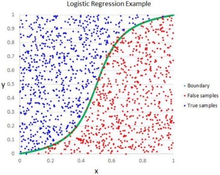
2b: Logistic regression
Below is a questionable illustration of logistic regression. [Image source is here]. Explain why the illustration has problems (1-3 sentences).