Last modified: 2020-12-01 09:40
Status: RELEASED.
Due date: Wed. Dec. 2 at 11:59PM AoE (Anywhere on Earth) (Thu 12/3 at 07:59am in Boston)
Updates
-
2020-12-01 : CLARIFIED in Task 6(i) what to report in Table 6 for the periodic nearest neighbor baseline on train+valid dataset
-
2020-11-25 : FIX to doctests updated to sqexp_kernel.py in starter code repo
Overview
In this HW, you'll complete the following:
Part I: Concept Questions (25% of your grade)
- Problem 0 has conceptual questions about SVMs
- Problem 1 has conceptual questions about PCA
Part II: Case Study on Kernel Methods for Temperature Forecasting
- Problem 2 has coding tasks (25% of your grade)
-
- You'll edit starter code in .py files.
-
Problems 3-6 are analysis and implementation tasks (50% of your grade)
-
- You'll implement tasks in a Jupyter notebook and produce plots and tables for a report
Turn-in links:
- PDF report turned in to: https://www.gradescope.com/courses/173055/assignments/859942/
- ZIP file of source code turned in to: https://www.gradescope.com/courses/173055/assignments/859941/
- Finally, complete your reflection here: https://docs.google.com/forms/d/1cBsuzUsTZ_moOKOtNaMMbuMlkoNmrrnIFIYTddVs73w
Files to Turn In:
PDF report:
- Prepare a short PDF report (no more than 5 pages).
- This document will be manually graded.
- Can use your favorite report writing tool (Word or G Docs or LaTeX or ....)
- Should be human-readable. Do not include code. Do NOT just export a jupyter notebook to PDF.
- Should have each subproblem marked via the in-browser Gradescope annotation tool)
ZIP file of source code should contain:
- linear_kernel.py (will be autograded)
- sqexp_kernel.py (will be autograded)
- periodic_kernel.py (will be autograded)
- hw5.ipynb (just for completeness, will not be autograded but will be manually assessed if necessary.)
Evaluation Rubric:
See the PDF submission portal on Gradescope for the point values of each problem. Generally, tasks with more coding/effort will earn more potential points.
Jump to: Background Problem 0 Problem 1 Dataset Starter Code Problem 2 Problem 3 Problem 4 Problem 5 Problem 6
Background
To complete this HW, you'll need some knowledge from the following sessions of class:
- SVMs (day18)
- Kernel Methods (day19 and day20)
- PCA (day22)
Below, we have specified relevant kernel functions for feature vectors \(x \in \mathbb{R}^F\) of size \(F\).
Linear kernel or (dot product kernel)
This is the simplest kernel: just the dot product (aka inner product) of the two original feature vectors:
This kernel has no hyperparameters.
Squared-exponential kernel
This kernel signals its "similarity" by the squared distance between two feature vectors of size \(F\).
This kernel has one hyperparameter: the length-scale \(\ell > 0\).
We like the "length scale" hyperparameter because it is more interpretable on the scale of the observed features \(x\):
- A length scale of 1 means:
- --- if x and z are about 1 apart (1 in squared distance), they have modest similarity of \(e^{-1} = \frac{1}{e} = 0.36\)
-
--- if x and z are further than 3 apart, they have pretty negligible similarity: \(e^{-3} = \frac{1}{e^3} = 0.05\)
-
A length scale of 3 means:
- --- if x and z are about 3 apart (9 in squared distance), they have modest similarity of \(e^{-1} = \frac{1}{e} = 0.36\)
- --- if x and z are further than 9 apart, they have pretty negligible similarity: \(e^{-3} = \frac{1}{e^3} = 0.05\)
In other words, if we fix \(x\) and fix a length scale \(\ell\), it is only points \(z\) within say \(\pm 3 \ell\) of \(x\) that "matter" (all other points will have very low kernel function values and thus low similarity).
Other names: Sometimes this kernel is called a "radial basis function" kernel or "Gaussian" kernel.
Other parameterizations: Sometimes, this kernel written with an alternative hyperparameter \(\gamma = \frac{1}{\ell^2}\).
Periodic kernel
This kernel signals its "similarity" via a periodic function of two univariate values \(x\) and \(z\):
The hyperparameter \(p\) is the period, and the hyperparameter \(\ell\) is a length scale.
Under this kernel, given fixed \(x\), the values \(x+p\), \(x+2p\), \(x+3p\), ... are equally "similar" under this kernel.
This kernel was originally suggested by David MacKay in a 1998 paper
The plot below illustrates this kernel function at several possible hyperparameter values:
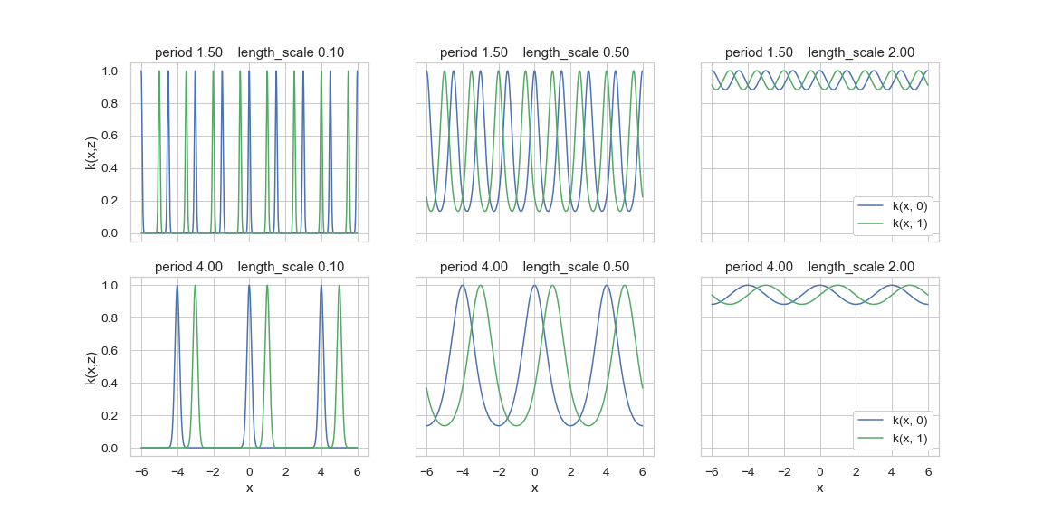
Visualization of the periodic kernel at length-scale and period hyperparameters.
Part I: HW5 Concept Questions
Problem 0: Conceptual Questions about SVMs
Throughout Problem 0, you can assume a binary classification task with \(N\) training examples, each with feature vector of size \(F\). Each feature is a numerical real value, and each feature has been separately normalized so the training set mean is 0 and variance is 1. You can guarantee that the maximum absolute value of any feature is at most 5.
Consider using a Support Vector Machine binary classifier with an RBF kernel in practice via the `SVC' implementation in sklearn. You could construct such a classifier as follows:
my_svm = svm.SVC(kernel='rbf', gamma=1.0, C=1.0)
Recall that the radial basis function (RBF) kernel is defined above in Background. We emphasize that sklearn's RBF kernel implementation uses the "gamma" parameterization of the RBF, with hyperparameter \(\gamma > 0\).
The hyperparameter \(C\) controls the relative strength of the hinge loss in the training objective, relative to another term that penalizes the complexity of the weight parameters.
For further details about what these hyperparameters mean, consult the documentation for sklearn.svm.SVC.
Please answer these questions as short answers in your PDF report:
0a: Describe a setting of the hyperparameters gamma and C that is sure to overfit to a typical training set and achieve zero training error.
Answer the following True/False question, providing one sentence of explanation.
0b True or False? Why?: An advantage of an SVM is that even with an L2 penalty on the weights, if we solve the "primal" optimization problem to train our model the optimal weight vector \(w \in \mathbb{R}^F\) (a vector with one entry per feature) will typically be sparse.
Problem 1: Conceptual Questions about Principal Components Analysis (PCA)
Consider Principal Components Analysis, which is described in the following resources:
- ISL textbook Chapter 10 (specifically sections 10.1 and 10.2)
- Jake VanderPlas' Python Data Science Handbook: https://jakevdp.github.io/PythonDataScienceHandbook/05.09-principal-component-analysis.html
You can assume you have a training dataset \(X\) with \(N\) examples, each one a feature vector with \(F\) features. You can imagine that it is a nutrition application, with many measurements describing a patient's height, weight, regular daily food consumption, and many other attributes.
Please answer the following questions about PCA, as short answers in your report PDF.
1a True or False? Why?: A recommended way to select the number of components \(K\) is to find the \(K\) value that minimizes reconstruction error on the training set. This choice will help us balance high-quality reconstructions and model complexity.
1b: Suppose you make two versions of your dataset with \(N\) examples and \(F > 1\) features. In the first version, you measure the height feature in centimeters. In the second, you convert the height feature to units of meters instead (but leave all other columns of data unchanged). Would the first K PCA components of these two datasets be the same, or different? Why?
1c: Stella has a training dataset \(X = \{ x_n \}_{n=1}^N\), which has \(N\) example feature vectors \(x_n\) each with \(F\) features. She applies PCA to her training set to learn a matrix \(W\) of shape \((K, F)\), where each row represents the basis vector for component \(k\).
She would like to project her test dataset \(X' = \{ x'_t \}_{t=1}^T\) using the same components \(W\). She remembers that she needs to center her data, so she applies the following 3 steps to project each \(F\)-dimensional test vector \(x'_t\) to a \(K\)-dimensional vector \(z'_t\):
Is this correct? If so, explain why. If not, explain what Stella should do differently.
Part II: HW5 Case Study: Kernelized Linear Regression for Temperature Forecasting
Dataset: Daily Minimum Temperature in Melbourne, Australia
In Problems 2-5, we'll try our new kernel regression skills to forecast the minimum-recorded outdoor temperature in Melbourne, Australia on a specific day in the future.
This is a supervised learning problem, where for each day (indexed by \(n\)) we have:
- Input \(x_n \in \mathbb{R}\), of type
float, is the number of fractional years between that day and Jan 1, 1985. - Output \(y_n \in \mathbb{R}\), of type
float, is the lowest temperature (in degrees Celsius) recorded on that day at a weather station in Melbourne
We're given a dataset of \(N=2400\) training examples (from 1981-1986) and \(T=730\) validation examples (from 1987 and 1988). All input,output pairs for both these datasets are shown here:
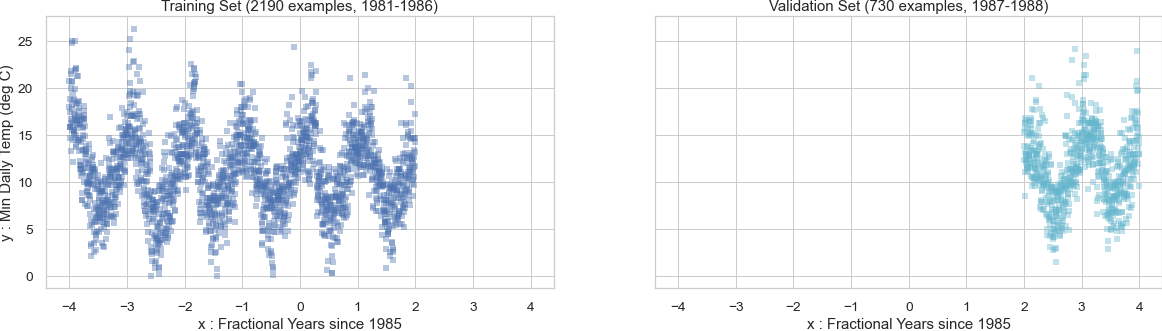
Training and validation datasets for the daily temperature dataset. These are the minimum daily temperatures recorded in Melbourne, Australia.
You are also given \(T=730\) test examples (from 1989-1990).
Your goal is to accurately predict the temperature on this test set.
Task: Regression
We want to build a forecasting regression model, so that we can predict the future temperature on some arbitrary date in the future (say on May 5th 3 years after the training data was collected).
Critically, to properly assess our model's forecasting ability, we will:
- Train parameters on a training set (our available dataset is from 1981-1986)
- Select hyperparameters on a validation dataset which comes from a time period in the future compared to the training set (1987-1988)
- Report our final performance on a test dataset from a time period in the future compared to the validation set (1989-1990).
Starter Code
See the hw5 folder of the public assignments repo for this class:
https://github.com/tufts-ml-courses/comp135-20f-assignments/tree/master/hw5
This starter code includes a notebook to help you get started on your analysis for Part II.
Problem 2: Implementation of Kernel Functions
Code Task A (30% of code grade): Implement calc_linear_kernel
See the Background on linear kernels.
You'll need to edit the starter code file: linear_kernel.py.
Code Task B (30% of code grade): Implement calc_sqexp_kernel
See the Background on squared exponential kernels.
You'll need to edit the starter code file: sqexp_kernel.py.
Code Task C (40% of code grade): Implement calc_periodic_kernel
See the Background on periodic kernels.
You'll need to edit the starter code file: periodic_kernel.py.
Problem 3: Linear Kernel + Ridge Regression
In this problem, you'll train and evaluate a linear kernel + ridge regression pipeline.
Follow the starter code notebook for detailed suggestions.
Task 3(i): Select Hyperparameters via Grid Search on Validation Set
Perform a grid search for these hyperparameters:
- ridgeRegressor
alphain np.logspace(-5, 5, 11)
Use the possible value grids specified in the starter notebook.
You want to find the value that maximizes mean absolute error on the validation set.
Task 3(ii): Fit Model with Best Hyperparameters to Train+Validation
Store this model for later use.
Figure 3 in your report
Plot the predictions of the best model, overlaid on the training and validation sets.
Short Answer 3 in your report
Reflect on Figure 3. Given what you know about this kernel, do the predictions make sense? How good is this model at interpolating? How good is this model at extrapolating?
Problem 4: Squared-Exponential Kernel + Ridge Regression
In this problem, you'll train and evaluate a sqexp kernel + ridge regression pipeline.
Follow the starter code notebook for detailed suggestions.
Task 4(i): Select Hyperparameters via Grid Search on Validation Set
Perform a grid search for these possible hyperparameters:
- sqexpKernel
length_scale - ridgeRegressor
alpha
Use the possible value grids specified in the starter notebook.
You want to find the value that maximizes mean absolute error on the validation set.
Task 4(ii): Fit Model with Best Hyperparameters to Train+Validation
Store this model for later use.
Figure 4 in your report
Plot the predictions of the best model, overlaid on the training and validation sets.
Short Answer 4 in your report
Reflect on Figure 4. Given what you know about this kernel, do the predictions make sense? How good is this model at interpolating? How good is this model at extrapolating?
Problem 5: Periodic Kernel + Ridge Regression
In this problem, you'll train and evaluate a periodic kernel + ridge regression pipeline.
Follow the starter code notebook for detailed suggestions.
Task 5(i): Select Hyperparameters via Grid Search on Validation Set
Perform a grid search for these possible hyperparameters:
- periodicKernel
period - periodicKernel
length_scale - ridgeRegressor
alpha
Use the possible value grids specified in the starter notebook.
You want to find the value that maximizes mean absolute error on the validation set.
Task 5(ii): Fit Model with Best Hyperparameters to Train+Validation
Store this model for later use.
Figure 5 in your report
Plot the predictions of the best model, overlaid on the training and validation sets.
Short Answer 5 in your report
Reflect on Figure 5. Given what you know about this kernel, do the predictions make sense? How good is this model at interpolating? How good is this model at extrapolating?
Problem 6: Final Showdown
In this problem, we'll compare the models we developed in Problems 3-5, in terms of performance on the test set.
Task 6(i): Baseline prediction: "Periodic Nearest Neighbor" regression
As a baseline prediction, consider predicting the temperature on some day in the test set by simply taking the median of all temperatures on the same calendar day on all available years in the development set (training plus validation together).
That is, if you want a prediction for December 2, 1989, simply consider the median of temperature values for:
- December 2, 1981 (the first year of the combined train+valid set)
- December 2, 1982
- ...
- December 2, 1987 (the last year of the combined train+valid set)
Remember that the x feature value is in units of fractional years, so subtracting 1 moves you 365 days behind, subtracting 2 moves you 2*365 days behind, etc..
Thus, if you want a baseline prediction for \(x = 6.8\), you can look up its "neighbors" by finding the examples whos \(x\) values are 6.8-2, 6.8-3, 6.8-4, 6.8-5, 6.8-6, 6.8-7, 6.8-8. This will give you the 7 values in the combined training+validation set which occur on the same day of the year. FYI There may be some off-by-one errors due to leap years (e.g. there may not be an exact match, but you should find a close match).
You should implement this baseline yourself (see starter notebook) and compute its mean absolute error.
Update 2020-12-01 Strategy to compute this baseline on train+valid set: For each train+valid example, take whichever years of 2 back, 3 back, 4 back, ... 8 back actually exist for your example in the dataset, and just use the median of those (e.g. to predict for a day in 1983 you would only the corresponding day in 1981, to predict for 1985 you would have 1981-83). If you cannot find any neighbors for an example, just omit that example from the calculation.
Table 6
Make a Table showing the performance on train+valid and test sets, for
Include a row for each of these:
- The linear KLR model from Figure 3
- The squared-exponential KLR model from Figure 4
- The periodic KLR model from Figure 5
- The periodic-nearest-neighbor baseline from Task 6(i)
- -- For this baseline, we care most about test set performance
- -- You can either skip the train+valid number, or use the strategy above to compute that.
Short Answer 6a
Reflect on the performance of the models in Table 6. Which one is best in terms of test-set performance? Why?
Short Answer 6b
Is the margin of improvement for the best temperature forecasting method over the linear model meaningful "in the real world"? To answer this think about both the units of this error, and how people use a temperature forecast. For example, suppose this forecast was the one published to the local population: would this improvement lead to changes in human experience (e.g. how people dress? how people plan their day?)