Introduction
Procedure calls and procedure calling conventions are among the deepest ideas in compiler construction. Since they implement recursion—a truly deep idea—the depth shouldn’t suprise you. Fortunately, the ideas themselves are simple. And because we control the SVM’s instruction set and procedure-calling convention, we will keep the implementation equally simple.
Recursive procedures work like this:
Every activation of a recursive procedure uses the same names for parameters and local variables.
And yet, in every activation, those names refer to different hardware locations.
The apparent inconsistency is resolved using a stack.
This idea is part of the curriculum in CS 40, and only one thing is different: in CS 40, the stack is a stack of memory locations. In the SVM, the stack is a stack of VM registers.
Location names and recursive functions: AMD64/SVM comparison
The best way to understand procedure calls, and to review your learning from CS 40, is to go deep on an example. We’ll use the naive, quadratic list-reversal function. In C code, it looks like this:
List reverse(List xs) {
  if (xs == NULL)
    return NULL;
  else
    return append(reverse(xs->cdr), list1(xs->car));
}
To understand how this recursive procedure is implemented, we’ll look at the AMD64 assembly code:1
reverse:
    # parameter xs passed in register %rdi
    pushq   %rbp                   # save the base pointer
    movq    %rsp, %rbp             # old stack ptr is new base ptr
    pushq   %rbx                   # save nonvolatile register
    subq    $24, %rsp              # allocate activation (shift stack)
    movq    %rdi, -24(%rbp)        # save parameter xs at -24(%rbp)
    cmpq    $0, -24(%rbp)          # xs == NULL ?
    jne     .L2                    # if not, go to L2
    movl    $0, %eax               # put 0 in return register
    jmp     .L3                    # .L3 restores context and returns
.L2:
    ... omitted for simplicity ...
    call    list1
    ... omitted for simplicity ...
    movq    -24(%rbp), %rax        # set %rax to xs
    movq    8(%rax), %rax          # set %rax to xs->cdr
    movq    %rax, %rdi             # pass xs->cdr to reverse
    call    reverse
    # result arrives in register %rax
    movq    %rbx, %rsi
    movq    %rax, %rdi
    # actual parameters passed in registers %rdi and %rsi
    call    append                 # tail call, not optimized!
.L3:
    addq    $24, %rsp              # restore the stack frame
    popq    %rbx                   # restore saved registers
    popq    %rbp
    ret                            # return
This code is worth analyzing, but to make the analysis easier, let’s also show my SVM code for the same procedure. The source code looks like this:
(define reverse (xs)
  (if (null? xs)
      '()
      (append (reverse (cdr xs) (list1 (car xs))))))
The SVM assembly code looks like this:
r0 := function (1 arguments) {
  ;; argument `xs` arrives in register `r1`
  r2 := null? r1
  if r2 goto L1
    ;; if xs is not empty
    r2 := global append
    r3 := global reverse
    r4 := cdr r1
    r3 := call r3 (r4)    ;; r3 := (reverse (cdr xs))
    r4 := global list1
    r5 := car r1
    r4 := call r4 (r5)    ;; r4 := (list1 (car xs))
    tailcall r2 (r3, r4)  ;; returns (append r3 r4)
  L1:
    ;; if xs is empty
    r0 := '()
    return r0
}
global reverse := r0
Comparing these two assembly-language sequences can tell us a lot about what is going on. Don’t try to digest all the details, but look over this comparison table, and remember what’s discussed here—then when it’s time to implement call, return, and tailcall, use it for reference.
| AMD64 | SVM |
|---|---|
Internally, the location of parameter xs has the same name in every activation (-24(%rbp)). |
Internally, the location of parameter xs has the same name in every activation (r1). |
The meaning of the name %rbp is changed at the beginning of the procedure (by the movq instruction on line 4). |
The meaning of the name r1 is changed before the procedure starts to run (by the call instruction that activates the procedure). |
The previous meaning of %rbp is restored before the procedure returns (by the popq instruction on line 28). |
The previous meaning of r1 is restored as the procedure returns (by the return instruction on line 17, or by the return instruction in append, which is tail called on line 13). |
The call instruction saves the return address on the call stack. |
The call instruction saves the return address on the call stack. |
Incoming parameters arrive in conventional registers (%rdi, %rsi, and so on). |
Incoming parameters arrive in conventional registers (r1, r2, and so on). |
Calls to functions list1, reverse, and append pass parameters in the same conventional registers at each call (%rdi, %rsi, and so on). |
Calls to functions list1, reverse, and append pass parameters in different registers at each call: reverse’s parameter is passed in r4, list1’s parameter is passed in r5, and append’s parameters are passed in r3 and r4. |
By AMD64 convention, the result from reverse must come back in register %rax, and to get it where it needs to go to append, the value has to be moved into %rdi (lines 20 and 22). |
The SVM can take a result into any register, so the call to reverse puts the result into r3 (line 9), and when it’s time to call append (line 13), the value is already where it needs to be—it doesn’t have to be moved. |
On the AMD64, the call to append produces its result in %eax, which is where reverse is also expected to produce its own result. So between lines 24 and 29, no work has to be done to get the result in the right place. This is an example of a small optimization. |
On the SVM, more optimization is possible. By making a tailcall to append on line 13, the assembly code not only ensures that the result of reverse is the result of append, it also instructs append to reuse its register window and activation record. The “push then pop” computation executed on the AMD64 is avoided here; that makes tailcall an optimized tail call.Given a suitable calling convention, any tail call can be optimized. Even when, as here, the call is not recursive. |
Location names and register windows
The big new idea in the SVM involves the names of locations. The C compiler uses locations on the stack, like -24(%rbp). We know that this stands for “the location 24 bytes below the base pointer,” but if we abstract a little bit, this phrase is just a name for the location. Every activation of reverse uses this same name, but in every activation, the name stands for a different location in hardware memory. In the SVM, we’re going to achieve exactly the same effect, but with one difference: we use register names. Using a single register name to mean a different location in each activation is made possible by hardware called register windows.
The idea of register windows is that the SVM has thousands of registers, but at any one time, code can only refer to a contiguous sequence of 256 registers. That sequence is the register window.
At a typical procedure call, the register window shifts toward higher-numbered registers. Here’s a picture of the call to list1 in function reverse:
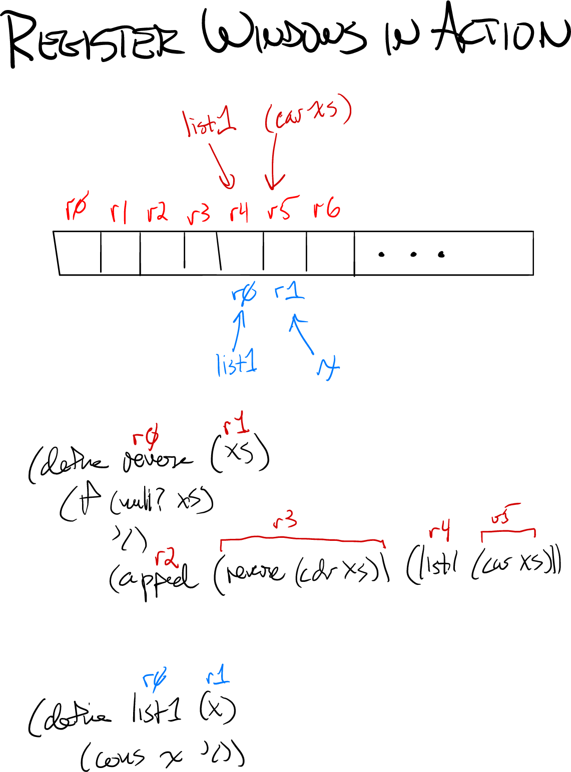
In the figure, here’s what’s going on:
The row of boxes outlined in black are the actual registers.
The names shown in red, above the registers, are the names used in function
reverse. The register window begins with the red r0.The names shown in blue, below the registers, are the names used in function
list1. The register window begins with the blue r0.
At the point where list1 is called, let’s look at reverse and see how each register is used.
According to the rules of our calling convention, register r0 holds the function being called (
reverse) and r1 holds the first parameter (xs).The code was in the process of setting up a call to
append, soappendis in register r2 and its first parameter is in r3.The code is about to call
list1, so the function about to be called is in register r4, and its actual parameter is in r5.
The next instruction to be executed is going to be
r4 := call r4 (r5)How can this work? Doesn’t the calling convention say the function goes in r0 and the first parameter in r1? Yes! When the VM sees the call instruction, it shifts the register window. The red r4 becomes the blue r0, the red r5 becomes the blue r1, and so on.
Imagine a piece of cardboard with a rectangular cutout 256 slots wide. That’s the window. At the call, the window slides 4 slots to the right. One beauty of this approach is that reverse can keep its private information in red registers r0 to r3, and nothing bad can ever happen to them, because they are inaccessible. Function list1 does not even have names for those registers.
In your VM, the easy way to implement register windows is to keep a pointer to register 0. A reference to a numbered register is implemented by an indexing operation from that pointer.
Hardware register windows: History and commentary
At the dawn of the microprocessor era in the 1970s, the circuits needed to build fast registers were so expensive that many processors didn’t have them. Early microprocessors had only two real registers (a program counter and a stack pointer). The Intel x86 architecture had a full eight general-purpose registers. Wow!
But from the poor compiler’s point of view, 8 registers aren’t a lot. The compiler has to figure out how to manage all of its local variables and temporary data using only 8 registers. This problem is called register allocation, and is one of the hardest problems in compilation. Many compiler courses, like this one, punt on register allocation—perhaps outsourcing it to LLVM.
By the middle 1980s, hardware had advanced enough that new instruction-set designs, like ARM and MIPS, supported 16 or even 32 general-purpose registers. (That’s why AMD64 is so much better than x86—it has twice as many registers.) And hardware kept getting better, and suddenly we had another problem: we started running out of space for register names. With 32 registers, an ADD instruction with three registers might spend 15 bits of the instruction encoding just to encode register names. It started to look like we couldn’t have more registers just because we couldn’t find bits in the instruction word. And then engineers at Berkeley and Sun had a brilliant idea: suppose we build hardware with more registers than we can actually name at one time? And we could change the names at will, so in different parts of the program, we could use the same names for different registers. That is the idea of register windows.
The register-windowed architecture with the largest commercial footprint was undoubtedly the SPARC. It provided 8 “global” registers along with a 24-register window that could be shifted in multiples of 16. This architecture made it pretty easy to build in, say, 72 or 80 hardware registers even though the instruction word could name only 32 registers.
Hardware register windows looked like a cool idea, but only for a brief era: hardware had enough transistors that it could support extra registers, but not so many that the hardware could basically remap instruction references into big, internal register numbers (which is the case today). That era lasted about 15 years: the amount of time that elapsed between the announcement of the SPARC architecture and the announcement of the AMD64 architecture. AMD64 updated the Intel platform from 8 registers to 16 registers. 16 registers are just good enough for most purposes, and Intel’s fabrication prowess, combined with the dominance of Microsoft Windows, eventually rendered the architectural insights of the 1980s and 1990s commercially irrelevant. Desktop and server applications are stuck with AMD64: a classic Worse is Better situation.
But for a virtual machine, register windows are still a superb choice.
Implementing functions and calls
Sliding the register window is only part of implementing a function call. To understand the rest, let’s start with what the VM needs to know about a function:
- What sequence of instructions it wants to execute
- The number of registers it uses
- How many parameters it is expecting
This information is part of the representation of a struct VMFunction defined in header file value.h. The information is used as follows:
The instruction sequence is what
vmrunstarts executing when a function is called. It can be stored in the VM’s state data structure or just cached in a local variable ofvmrun.The number of registers is used to make sure that the VM’s representation of the complete register file has already allocated a slot for each register that might be used. That is, the VM ensures that every register that might be used is mapped.
The number of parameters the function expects2 is compared with the number of actual parameters at the call site. If they match, all is well. otherwise, the VM has three options:
It can implement a \(\mu\)Scheme-style semantics in which a mismatch in the number of parameters causes a run-time error. This is the semantics of vScheme and is the default behavior.
It can implement a semantics in which the actual parameters are “adjusted” to fit the function: extra actual parameters are discarded, and missing actual parameters are initialized to
nil. This is the semantics of Lua; it is available to implement for depth points.It can implement a partial-application semantics in which functions are automatically curried:
If there are extra actual parameters, the VM calls the function with only as many parameters as it is expecting, then applies the result to the extra parameters.
If there are missing actual parameters, the VM creates a closure that expects to receive the missing parameters, then activates the original function.
This is the semantics of Haskell and OCaml; it is available to implement for depth points.
Once a function’s information is known, the function can be called. And when its code starts to run, the function object itself is in register r0, and its actual parameters (1 to \(n\)) are in registers r1 to r\(n\). Higher-numbered registers (registers \(n+1\) to 255) contain unspecified values and are available for any purpose.
The call stack
A hardware implementation of procedure calls has to save the calling context in registers and memory. But in our SVM, we introduce additional state just for managing calls. (Real hardware has such state as well, but it is buried in caches and optimizations; it’s not visible in the instruction-set architecture.) That state is a stack, and for each activation it records the following information:
- Where the register window is
- Where the suspended execution is slated to resume
- What register in the caller is expecting to receive the result (the destination register)
This information is stored in a record of type struct Activation, which you will define in header file vmstack.h. In the operational semantics, the record is written as (R, I₁•I₂, r), where R represents the register window, I₁•I₂ represents the instruction stream and program counter, and r represents the destination register. These records are organized into a finite array, which the VM manages as a stack.
The three instructions
The call stack is manipulated by three instructions: call, return, and tail call.
To call a function f, the caller places f’s value in register \(r[k]\), and it places N actual parameters in registers \(r[k+1]\) through \(r[k+N]\). It then executes a call instruction with the \(X\) field set to \(x\) (naming a result register), the Y field set to \(k\), and the Z field set to \(k+N\). The call is assumed to kill registers \(r[k]\) and higher—that is, all the registers in the callee’s window. When the call terminates, the returned value is in register \(r[x]\).
To implement the call, the VM pushes a struct Activation on the call stack, slides the register window, and activates the new function.
An active function f terminates in one of two ways:
It returns a value. There must be an activation on the stack, which tells where the return value is expected. The register window slides; the returned value gets placed where the caller requested it; the instruction stream and program counter are restored to their values before the call, and the
struct Activationis popped off the call stack.It makes a tail call to another function
g. This looks like an ordinary call with these changes:The register window doesn’t move. Instead,
gis copied into registerr0, and the actual parameters (if any) are copied intor1,r2, and so on.Nothing happens to the call stack.
Once you’ve implemented a register window, a call stack, and the three instructions, you’ve implemented procedure calls.