CP3: Gaussian Mixture Models

Last modified: 2020-04-01 15:07

Due date: Wed. Apr. 1, 2020 at 11:59pm (late deadline Sun Apr. 5 11:59pm).

Status: RELEASED.

Updates:

• 2020-04-01: Bug fix in suggested assert statement in EM starter code
• 2020-03-30: Fixed typo in calc_EM_loss coding task description
• 2020-03-26: Updated turn-in links to gradescope. Autograder is ready!

What to turn in:

• PDF write up: https://www.gradescope.com/courses/82862/assignments/414798/
• ZIP file of source code: https://www.gradescope.com/courses/82862/assignments/414797

Your ZIP file should include

• All starter code .py files (with your edits) (in the top-level directory)
• These will be auto-graded. Be sure to check gradescope test results for immediate feedback.

Your PDF should include (in order):

• Your full name
• Collaboration statement
• About how many hours did you spend (coding, asking for help, writing it up)?
• Problem 1 figures and short answers
• Problem 2 figure and short answers

Questions?: Post to the cp3 topic on the discussion forums.

Jump to: Problem 1   Problem 2   Starter Code

Overview and Background

In this coding practical, we will implement 2 possible algorithms for learning the parameters (weights, means, and variances) of a Gaussian mixture model:

• LBFGS Gradient descent (Problem 1)
• Expectation Maximization (Problem 2)

The problems below will try to address several key practical questions:

• How sensitive are methods to initialization?
• How can we effectively select the number of components?
• What kind of structure can GMMs uncover within a dataset?

Probabilistic Model: Goals and Assumptions

We are given \(N\) data examples of observed feature vectors: \(\{ x_n \}_{n=1}^N\), with \(x_n \in \mathbb{R}^D\).

Our goal for model fitting is to learn a flexible probability distribution over \(x\), \(p(x_n)\).

Likelihood model

We model the \(N\) observed outputs \(x = \{x_n \}_{n=1}^N\) with a \(K\)-component Gaussian mixture model, which has the following likelihood (NB: this is the formulation without latent variables):

We have three kinds of parameters:

• Component-specific mixture weights: \(\pi = [ \pi_1 ~\pi_2 ~\pi_3 \ldots ~\pi_K]\)

• Component-specific per-dimension means: \(\mu = \{\mu_k \}_{k=1}^K\), \(\mu_k \in \mathbb{R}^D\)

• Component-specific per-dimension standard deviations: \(\sigma = \{ \sigma_k \}\), \(\sigma_k = [ \sigma_{k1} ~ \sigma_{k2} ~ \ldots ~ \sigma_{kD} ]\). Each standard deviation must be positive: \(\sigma_{kd} > 0\).

We emphasize that throughout this CP problem set, the variance is controlled by a separate parameter for each data dimension (indexed by \(d\)), and thus there is assumed no correlation between distinct dimensions of the vector \(x_n\).

Training Goal: Maximize penalized likelihood

We wish to maximize a penalized likelihood, or equivalently, minimize the penalized negative log likelihood:

where the likelihood has been defined above, and the penalty term is designed to avoid the degeneracies of unpenalized maximum likelihood training of GMMs where some components can gain "infinite" likelihood by sending \(\sigma_k \rightarrow 0\).

We will use the following penalty on parameters that control the variance:

with two parameters: \(m > 0\) and \(s > 0\).

We will call \(m\) the "mode" of the variance penalty, because if the penalty were the only thing optimized, we would prefer to set \(\sigma^2 = m\).

We will call \(s\) the "spread" or maybe "flatness" of the variance penalty, because larger values make the region around the mode flatter and flatter.

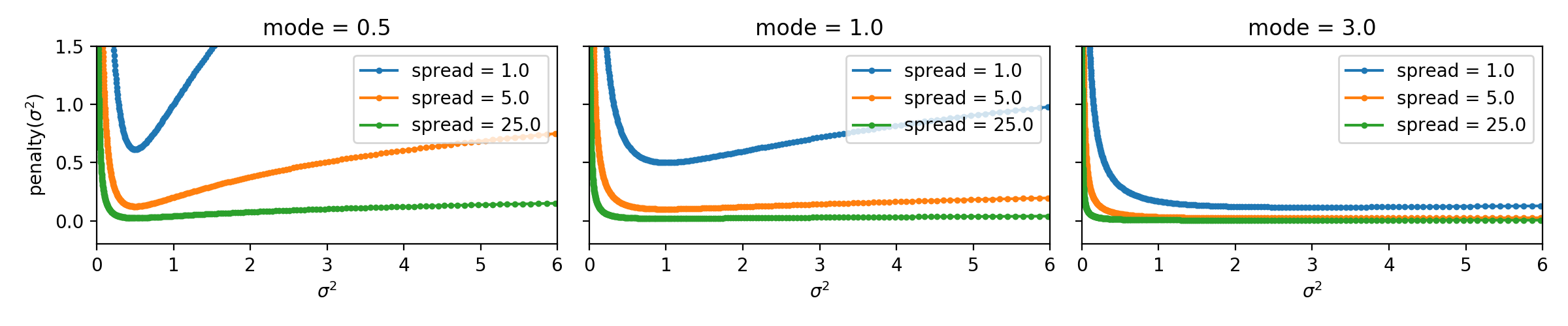
Plot of penalty function vs sigma. See `stddev_penalty_function.py` in starter code.

Technical Challenge: Transform to unconstrained parameters

For gradient-based methods to work effectively, we cannot just naively take gradient steps of constrained parameters like the vector \(\pi\) (which must live in \(\Delta^K\)) or the scalar standard deviations \(\sigma_{kd}\) (which must live in the positive reals).

Mixture weight transformation : To handle the constrained vector \(\pi \in \Delta^K\), we replace it with a deterministic transformation \(T\) which produces an unconstrained vector \(\rho \in \mathbb{R}^K\) via the following transformation:

Recall that the logsumexp function computes \(\log \sum_{k} e^{\rho_k}\) in a numerically stable way.

Throughout, in our code implementation we will work directly with the vector \(\log \pi\) (the elementwise application of the logarithm to the length-\(K\) vector \(\pi\)).

Variance transformation : To handle the constrained vector \(\sigma_k \in \mathbb{R}_+^D\) (the set of vectors with all positive entries), we use the following deterministic transformation \(U\) to produce an unconstrained vector \(\nu_k \in \mathbb{R}^D\):

where the softplus function and its inverse are defined as:

We can guarantee that \(\text{softplus}(a) > 0\) for any \(a \in \mathbb{R}\), as required to produce a valid variance.

Many other transforms could have been used. One reason to use the softplus instead of just "exp/log" is that we want small changes in \(\nu\) (e.g. after a small gradient update) to not produce big changes in \(\pi\). Softmax has a much more linear relationship between \(\nu\) and \(\sigma\) than the exp would.

Algorithm #1 ("LBFGS"): Gradient Descent via L-BFGS

We will consider a "gold standard" first-order gradient descent method called "L-BFGS" limited-memory Broyden–Fletcher–Goldfarb–Shanno algorithm, which uses first-order gradients computed at every iteration plus intelligent tracking of previous gradient steps to obtain an affordable approximation to the Hessian required for Newton-Raphson second order steps.

Why L-BFGS? Often, its Newton-method-inspired step-size selection is far more effective than just doing steepest descent (e.g. \(v \gets v - \epsilon \text{grad}(v)\)) or other first-order methods where you'd need to tune your step size carefully.

The algorithm proceeds as follows:

• Initialize the parameters \(\pi, \mu, \sigma\) at random

• Transform to unconstrained parameters: \(\rho = T(\pi), \nu = U(\sigma)\).

• Pack all unconstrained parameters into one parameter vector, which will be initial value at iteration 0: \(v^0 = [\rho, \mu, \nu]\)

• Prepare two functions that can take as input the unconstrained vector \(v\): the loss and the gradient: \(\text{calc_loss}\) and \(\text{calc_grad}\)

• Repeat at every iteration \(t \in 1, 2, \ldots T\):

• • Compute gradient vector \(g^{t-1} \gets \text{calc_grad}(v^{t-1})\)
• • Update parameter vector \(v^t \gets \text{LBFGS_update}(v^{t-1}, g^{t-1})\)

• Unpack the final unconstrained params: \(\rho, \mu, \nu \gets v^{T}\)

• return final constrained parameters: \(\pi = T^{-1}(\rho), \mu, \sigma = U^{-1}(\nu)\).

Naturally, you could check for some convergence criteria after every iteration, and terminate early.

Implementation Details for LBFGS

To implement LBFGS, you will need to implement the calc_loss function.

After that however, your starter code will pretty much do the rest.

Gradients with autograd

Because we are using the autograd module, which provides automatic differentiation capability, you do NOT need to implement a calc_grad function by hand! Instead, if you have defined calc_loss correctly, you can just build a function to compute the gradient by calling: calc_grad = autograd.grad(calc_loss). See the starter code!

If you have never used autograd before, it is pretty easy, just write numpy code as normal and autograd does the rest. You just make sure you use the ag_np module, imported like so import autograd.numpy as ag_np. This module is already installed in your spr_2020s_env python environment.

For more help on autograd, see the package README, tutorial TLDR, and/or this tutorial from Tufts COMP 135 (which you should only need the first few exercises from): https://github.com/tufts-ml-courses/comp135-19s-assignments/blob/master/labs/IntroToAutogradAndBackpropForNNets.ipynb

LBFGS with scipy.optimize.minimize

You should not implement the LBFGS update yourself. You should use scipy.optimize.minimize, with the setting method=l-bfgs-b. See starter code.

Transformations with starter code

You should also not implement the parameter transformation functions either. See starter code and use the transformations there.

Algorithm #2 ("EM"): Expectation Maximization

Next, we will consider the EM algorithm, which is outlined in Bishop's PRML textbook chapter 9 and in our lecture in day 16 (see notes in day16.pdf).

The algorithm proceeds as follows:

• Initialize the parameters \(\pi, \mu, \sigma\) at random

• Repeat at every iteration \(t \in 1, 2, \ldots T\):

• • for each example \(n \in 1, 2, \ldots N\):
• • • E step for assignments: Update assignment probability vector \(r_n\) given current parameters \(\pi, \mu, \sigma\):

• • for each component \(k \in 1, 2, \ldots K\):
• • • M step for weights: Update \(\pi_k\) given \(x, r\): \(\quad \pi_k = \frac{\sum_{n} r_{nk}}{N}\)
• • • M step for means: Update each dim. \(\mu_{kd}\) given \(x, r\): \(\quad \mu_{kd} = \frac{\sum_{n} r_{nk} x_{nd}}{ \sum_{n} r_{nk}}\)
• • • M step for variances: Update each dim. \(\sigma_{kd}\) given \(x, r, \mu_{kd}\): \(\quad \sigma^2_{kd} = \frac{\frac{1}{s \cdot m} + \sum_{n} r_{nk} (x_{nd} - \mu_{kd})^2}{\frac{1}{s \cdot m^2} + \sum_{n} r_{nk}}\)

where we have done the math to incorporate the penalty into the \(\sigma\) update. Recall that \(m\) is the mode and \(s\) is the spread of the penalty term.

We can show that this algorithm minimizes a principled objective function involving a negative expected log complete likelihood, the negative entropy of \(q(z_n | r_n)\), and the penalty term defined above. The first two terms of this objective are worked out for the \(D=1\) case on page 9 of day16.pdf), though beware that math is maximization rather than minimization.

Hints for Implementation

Scalability : Avoid for loops as much as possible. Anything you can do with predefined numpy functions that are vectorized (e.g. using my_sum = np.sum(vec_K) instead of for v in vec_K: my_sum += v), please do so. In our solutions, we have 0 for loops over examples \(n\), and usually within each routine only one for loop over clusters \(k\). Recommended reading: https://realpython.com/numpy-array-programming/.

Numerical stability : You should probably try to use the logsumexp trick to compute the GMMPDF likelihood. The product of many normal PDFs could cause problematic underflow otherwise. Better to compute the sum of log PDFs, and then use the logsumexp to compute the total log probability.

Starter Code

You can find the starter code and datasets in the course Github repository here:

https://github.com/tufts-ml-courses/comp136-spr-20s-assignments/tree/master/cp3

Starter Code Installation Notes:

• If you have the spr_2020s_env installed from CP1, you don't need to do anything else.

• If not, follow directions in the README for how to install the required Python packages

Dataset

Your goal will be to train mixture models for images of short or long-sleeve shirts ("tops") from the FashionMNIST dataset.

Inside the data/ folder of the starter code repo, you will find several CSV files:

• tops-20x20flattened_train.csv : Training set of 3000 images (1000 from each category)
• tops-20x20flattened_valid.csv : Validation set of 1500 images (500 from each category)
• tops-20x20flattened_test.csv : Test set of 1500 images (500 from each category)

These represent a targeted subset of the FashionMNIST dataset, consisting of 20 pixel x 20 pixel images of 3 categories from Fashion MNIST: "t-shirt", "pullover", and "shirt", illustrated below:

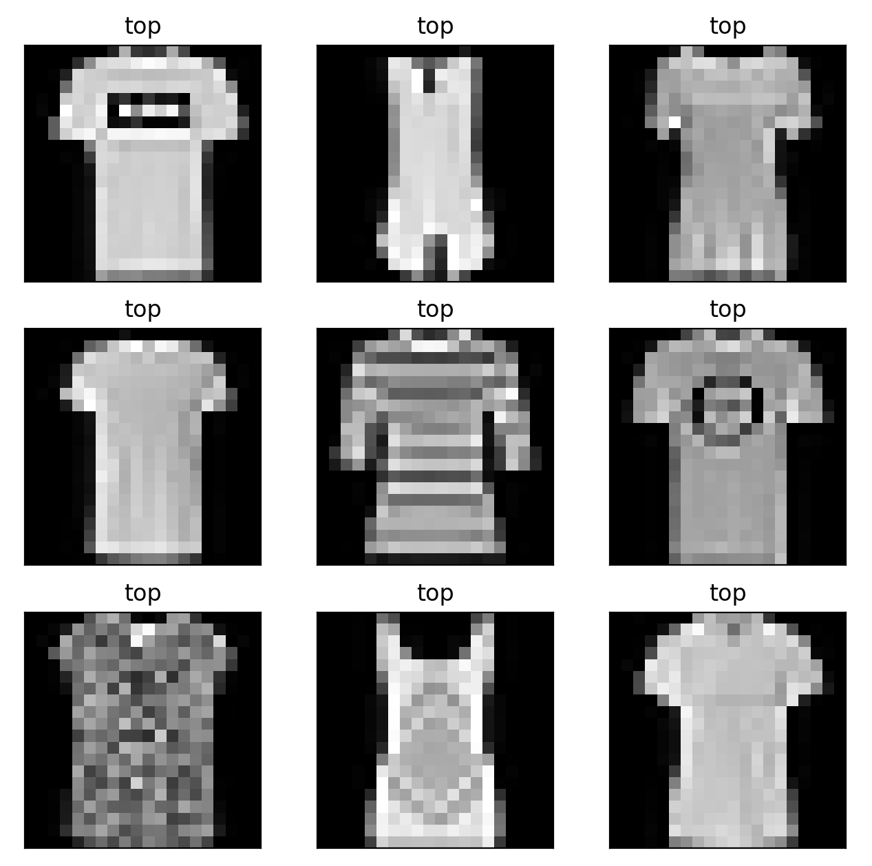
Tops category

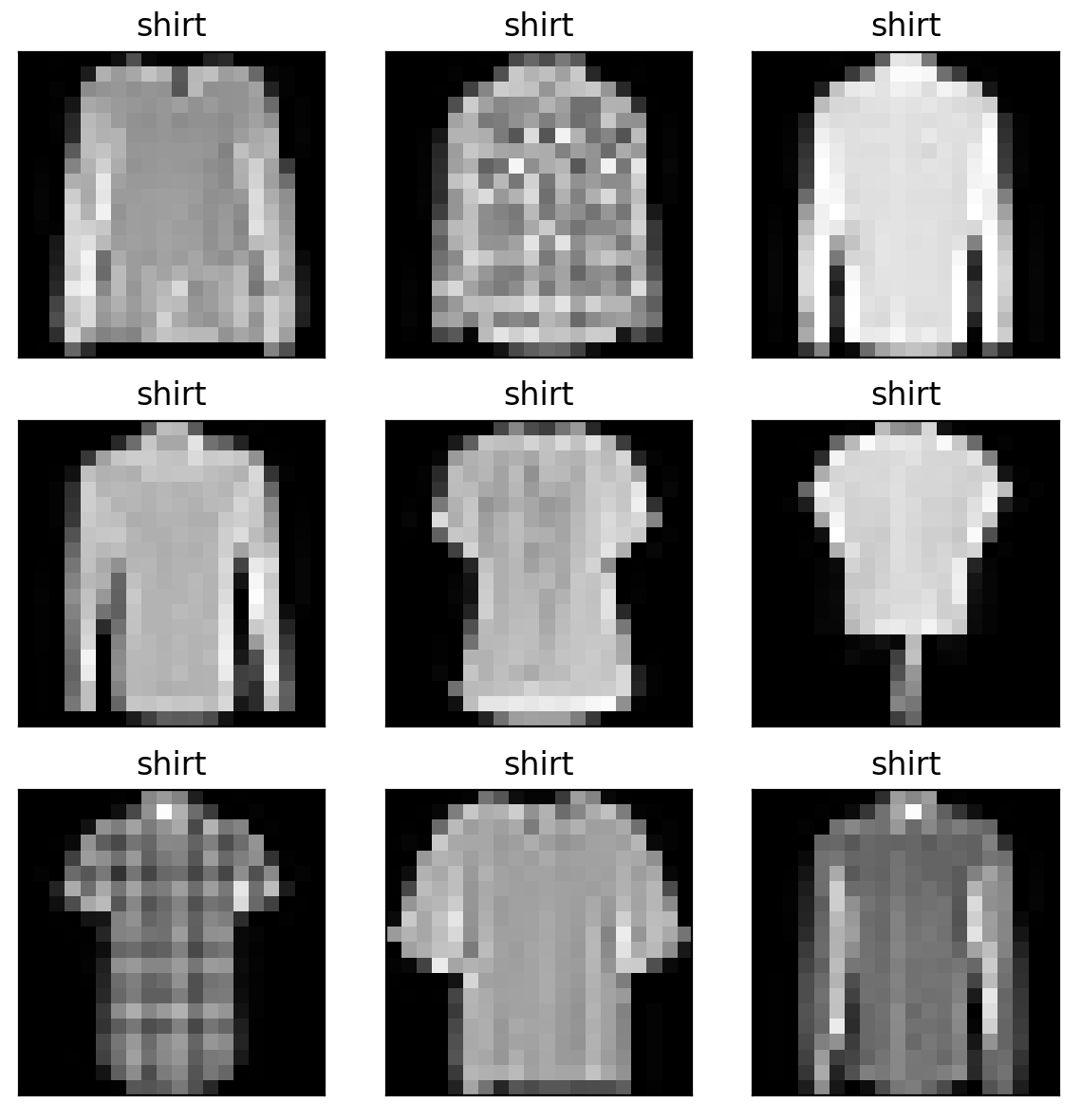
Shirts category

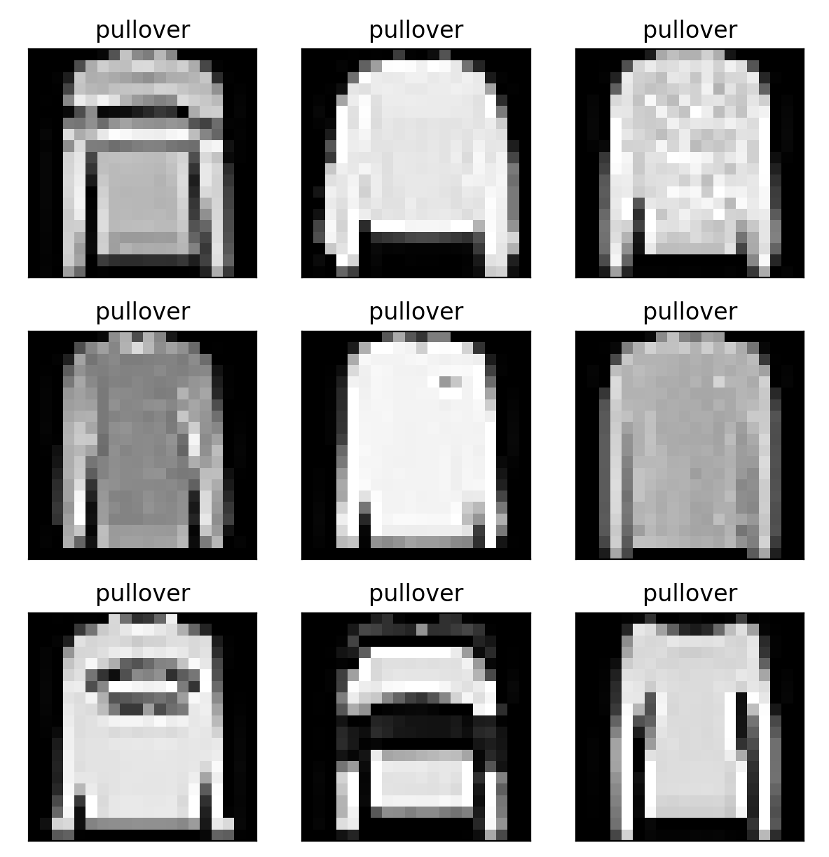
Pullover category

To represent each image, we took the 20x20 grayscale image, rescaled each pixel's intensity value to be a float between -1.0 and +1.0, and then "flattened" the image into a feature vector of size 400. Each row of the CSV file represents one "flattened" 20x20 pixel image.

Problem 1: LBFGS for GMMs

In problem 1, we will implement L-BFGS gradient descent for training GMMs, using the penalized ML loss function above.

We will then examine how well this procedure trains models on a limited computational budget.

• Look at likelihoods of heldout data
• Interpret the learned components by inspecting learned weights, means and variances

Tasks for Code Implementation

(All these steps will be evaluated by Autograder)

WRITING CODE 1(i) Implement the TODOs in the calc_negative_log_likelihood method of starter code found in calc_gmm_negative_log_likelihood.py

WRITING CODE 1(ii) Implement the TODOs in the fit method of the starter code class GMM_PenalizedMLEstimator_LBFGS, which define the overall loss and the validation performance metrics.

USING CODE 1(iii) Use the provided train_LBFGS_gmm_with_many_runs.py. This considers several values of K: 1, 4, 8, 16. For each value of K, initialize a GMM using the provided generate_initial_parameters function with a specified random seed, and train for 25 LBFGS iterations (a limited budget by design, should take ~10-30 minutes). Repeat for all the 5 different random seeds provided in the starter code (1001, 2001, 3001, 4001, 5001).

USING CODE 1(iv) Among all training runs for K, select the single run that has the best validation likelihood and mark this as the "best" run.

Tasks for Report PDF

1a: FIGURE: Training Loss and Validation Likelihood vs. Iteration, across K values. Using your pretrained models above, use the "plot_history_for_many_runs.py" script to make a figure with two rows and several columns (one column for each value of K). In the top row of panels, make a line plot of the training loss (per pixel) versus iteration, with a separate line for each random seed. In the bottom row of panels, make a line plot of the validation score (negative log likelihood per pixel) versus iteration, with a separate line for each random seed.

1b: FIGURE: Visualization of best LBFGS result with K=4 Using the best run with K=4, make a figure showing the visualization of the learned GMM parameters. Provide a caption that tries to interpret the learned parameters (1-2 sentences).

1c: FIGURE: Visualization of best LBFGS result with K=16 Using the best run with K=16, make a figure showing the visualization of the learned GMM parameters. Provide a caption that tries to interpret the learned parameters (1-2 sentences).

Problem 2: EM for GMMs

In problem 2, we will implement EM coordinate descent for training GMMs, using the penalized ML loss function above.

Tasks for Code Implementation

(All code steps will be evaluated by Autograder)

WRITING CODE 2(i) Implement the calc_EM_loss method of starter code class GMM_PenalizedMLEstimator_EM.

WRITING CODE 2(ii) Implement the estep__update_r_NK method of starter code class GMM_PenalizedMLEstimator_EM.

WRITING CODE 2(iii) Implement each of the mstep__update methods in starter code class GMM_PenalizedMLEstimator_EM.

WRITING CODE 2(iv) Implement the remaining TODOs in the fit method of starter code class GMM_PenalizedMLEstimator_EM.

USING CODE 2(v) Use the provided train_EM_gmm_with_many_runs.py script. This considers several values of K: 1, 4, 8, 16. For each value of K, initialize a GMM using the provided generate_initial_parameters function with a specified random seed, and train for 25 EM iterations (a limited budget by design, should take ~5-30 minutes). Repeat for all the 5 different random seeds provided in the starter code (1001, 2001, 3001, 4001, 5001).

USING CODE 2(vi) Among all EM training runs for each K, select the single run that has the best validation likelihood and mark this as the "best" run.

Tasks for Report PDF

2a: FIGURE: EM Training Loss and Validation Likelihood vs. Iteration, across K values. Using your pretrained EM models from 2(v) above, use the "plot_history_for_many_runs.py" script to make a figure with two rows and several columns (one column for each value of K). In the top row of panels, make a line plot of the training loss (per pixel) versus iteration, with a separate line for each random seed. In the bottom row of panels, make a line plot of the validation score (negative log likelihood per pixel) versus iteration, with a separate line for each random seed.

2b: FIGURE: Visualization of best EM result with K=4 Using the best run with K=4, make a figure showing the visualization of the learned GMM parameters. Provide a caption that tries to interpret the learned parameters (1-2 sentences).

2c: FIGURE: Visualization of best EM result with K=16 Using the best run with K=16, make a figure showing the visualization of the learned GMM parameters. Provide a caption that tries to interpret the learned parameters (1-2 sentences).

2d: SHORT ANSWER: Reflect on the K=1 runs. How did you result differ across runs? What would you expect to happen when running EM with K=1 on any dataset?

2e: SHORT ANSWER: Reflect on the differences between EM and LBFGS. Which method seems to work more reliably? Why do you think this is?

2f: SHORT ANSWER: Compute and report the negative log likelihood per pixel on the test set, for the best EM-trained models with K=4, K=8, and K=16 (you'll have to write your own code to load this test set from data/ and determine the likelihood). Is one K value noticeably better? How does this comparison on the test dataset compare with the same on validation dataset?