Last modified: 2019-10-21 16:10
MNIST + Autoencoders
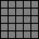
Before Training
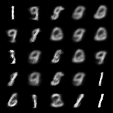
At Epoch 1
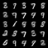
After many epochs
Due date: Mon. October 21, 2019 at 11:59 PM
Status: Released
What to turn in:
- PDF report: https://www.gradescope.com/courses/61382/assignments/277482/
- ZIP file of source code: https://www.gradescope.com/courses/61382/assignments/277436/
Your PDF should include (in order):
- Your full name
- Collaboration statement
- About how many hours did you spend (coding, asking for help, writing it up)?
- About how many hours did your CPU spend on Problem 2?
- Problem 1 answer (with parts clearly labeled in the PDF itself and marked via the gradescope annotation tool)
- Problem 2 answer (with parts clearly labeled in the PDF itself and marked via the gradescope annotation tool)
Your ZIP file should include
- Any code you developed, as .py or .ipynb (Jupyter notebook) files.
Questions?: Post to the hw4 topic on the discussion forums.
Jump to: Problem 1 Problem 2 Debugging Tips
Software Notes
Use the starter code: https://github.com/tufts-ml-courses/comp150-bdl-19f-assignments/tree/master/homeworks/hw4
Make sure you have latest version of the starter code.
Latest updates (with timestamp):
- 20191011 20:00 Released code
You'll need to fill in all the TODO statements to make it work!
Requires: PyTorch
You'll need to have a working install of PyTorch to use the starter code.
This is part of the bdl_2019f_env https://www.cs.tufts.edu/comp/150BDL/2019f/setup_python_env.html
Background
In class, we have learned about approximating posteriors with variational inference, using the reparameterization trick for VI (e.g. in the Bayes-by-Backprop algorithm), and deep generative models for images using variational autoencoders. It's now time to try to bring these ideas together.
In HW4, you will combine these ideas together to train models that can generate images of handwritten digits from the MNIST dataset. First, you'll directly train autoencoders for images via maximum likelihood methods. Next, you'll compare these results to a more Bayesian approach, the VAE.
Data
We consider the MNIST dataset of carefully cropped images of hand-written digits. We will use a version where each image is a 28 x 28 binary image. For more background, see: https://en.wikipedia.org/wiki/MNIST_database.
We observe \(N=60000\) total training examples of images of hand-written digits. We'll index each image with \(n\).
Each image can be defined by a 784-dimensional binary vector called \(x_n\). To make things more general, we can say that \(x_n\) has size \(P\), where P=784 in the case of MNIST and in general would could the number of pixels in the image.
FYI, we can always reshape the vector \(x_n\) into a 28x28 binary image for display purposes. But it'll be easiest to work with a flat vector.
Neural Networks : Ingredients for Probabilistic Modeling
Decoder Neural Network: From Code Vector to Image
We will use a decoder feed-forward neural network to map each possible 2D code \(z_n\) to a 784-dim vector of probabilities (each entry is a real value between 0 and 1).
We will always denote the parameters (weights and biases) of the decoder as a vector \(\theta\). The size of this vector depends on the architecture.
Possible Decoder Architectures
Decoder Arch. D1-X:
- 1 Hidden Layer with X units + ReLU activation
- 1 Output Layer with 784 units + sigmoid activation (so each entry is between 0.0 and 1.0)
Encoder Neural Network: From Image to Code Vector
We will use an encoder feed-forward neural network to map each possible 784-dimensional binary image vector to a specific possible 2D code vector \(z_n\).
Possible Encoder Architectures
Encoder Arch. E1-X:
- 1 Hidden Layer with X units + ReLU activation
- 1 Output Layer with 2 units + no activation (so output is real-valued)
Goals of Model Fitting
Our goal in fitting an autoencoder to data is twofold. First, we want to train decoder parameters \(\theta\) and encoder parameters \(\phi\) to have accurate reconstructions. Second, we wish to build a probabilistic model on top of an autoencoder, so that we can reason about our uncertainty over the code space.
For goal 1, we will simply produce a point estimate of the encoder and decoder parameters \(\theta\) (following the principle of minimizing reconstruction error).
For goal 2, we'd like to be "more Bayesian", so we'll assume a full generative model for our data. This model has a prior on code values and a likelihood of producing a data vector given a code vector. Given observed data, in the usual way we can write a posterior over the code values, and then approximate this posterior using variational inference. In this way, both our encoder and decoder are viewed as "stochastic" operations.
Goal 1 (Problem 1): Fitting an AE to Minimize Reconstruction Error
For this first goal, we will ignore the prior. We wish to find the decoder and encoder parameters that, for the training data at hand, minimize reconstruction error.
Reconstructed probability vector \(\tilde{x}\)
Given an input data vector \(x_n\), we can "reconstruct" it by encoding it to a code vector, then decoding that code vector. In math:
The result, \(\tilde{x}_n\), is still a vector the same size as \(x_n\). Under our chosen architectures, it is not binary but instead contains real values between 0.0 and 1.0.
Minimize Binary Cross Entropy (our chosen reconstruction error)
We wish to minimize the cross entropy, which is a cost function well-justified by information theory that you can read about on Wikipedia. The formula is:
This is a measure of error: a good autoencoder will have low "bce".
Maximize Bernoulli log likelihood
In fact, the above is equivalent to maximizing the logpdf of a Bernoulli likelihood that produces a positive binary value \(x_{np}\) with probability \(\tilde{x}_{np}\):
Note that this "likelihood" is not a valid probabilistic model (we cannot have \(\tilde{x}_n\) depend on \(x_n\) while \(x_n\) depends on \(\tilde{x}_n\)). But, it's still a way to set up an optimization problem.
We can solve the reconstruction optimization problem using modern gradient descent tools. In problem 1, you'll try out fitting AE models to minimize reconstruction error and see what tradeoffs might exist in terms of architectures and learning rates.
Goal 2 (Problem 2): Full Generative Model with an VAE Approximate Posterior
Prior on Codes \(z\) (Generative Model Step 1)
We assume that each image has a latent code vector \(z_n\) of size 2, so \(z_n \in \mathbb{R}^2\). The prior distribution over this vector's values is just a standard Normal:
Likelihood of Data given Code (Generative Model Step 2)
Given a decoder, we can write a probabilistic model for generating a data vector \(x_n\) given its code vector \(z_n\):
The ideal result of goal 2 would be a way to estimate the code-given-data posterior: \(p(z_n | x_n)\).
However, this posterior is difficult, even if we have good estimates of \(\theta\)! Why? The likelihood is non-linear, so the posterior does not belong to any known density family with easy-to-derive formulas for posterior parameter values.
To gain tractability, we'll try to solve a simpler problem. We will look at possible approximate posteriors that have more managable form.
We will assume that there is an independent Normal \(q\) distribution for each example \(n\). We will assume this Normal has a known fixed variance \(\sigma\) for all examples, and a mean parameter that is determined by an encoder neural network that is shared across all examples.
FYI this is a simpler approximation than in Kingma & Welling's paper (where the per-example variance depends on an additional 'encoder').
Here, the parameters \(\phi\) of the encoding network will be trained to provide the best possible encoding (bring the \(q(z_n | x_n)\) distribution as close as possible to the true posterior \(p(z_n | x_n)\)).
Variational Objective Function to Maximize
This objective function \(\mathcal{L}(\theta, \phi)\) takes in the encoder parameters \(\phi\) and decoder parameters \(\theta\), and produces a scalar real value.
The readings discuss how this function is a "lower bound" on the marginal likelihood (the "evidence") \(\log p(x | \theta) = \log \int_z p(x, z| \theta) dz\). We wish to find parameters that maximize this evidence lower bound (ELBO). The parameters include the generative model's parameters \(\theta\) and the parameters \(\phi\) for our approximate posterior.
VI Loss Function (Objective to Minimize)
Often, we are interested in framing inference as a minimization problem (not maximization). Esp. in deep learning, minimization is the common goal of optimization toolboxes. For example, PyTorch expects a loss function to minimize.
We can thus define that our "VI loss function" (what we want to minimize) is just -1.0 times the evidence lower bound objective above.
"VI loss function": \(-1.0 \cdot \mathcal{L}(\theta, \phi)\)
Training Optimization Problem for Goal 2
Our goal is to learn values for \(\theta, \phi\) that make the objective to minimize as small as possible. Here's the optimization problem:
We can then use:
- Monte Carlo methods to evaluate the objective function \(\mathcal{L}\)
- Reparameterization trick methods to estimate the gradient of \(\mathcal{L}\) with respect to \(\phi\) and \(\theta\)
These two ideas, together, allow us to fit this VAE model to data.
Problem 1: Fitting Autoencoders to MNIST to Maximize Likelihood
You can use the hw4starter_ae.py script to perform maximum likelihood estimation of the parameters of the encoder and decoder networks.
You'll need to train 3 separate models with 32, 128, and 512 hidden units (these size specifications are used by both encoder and decoder in the released code).
You'll need to adjust the learning rate --lr and potentially other keyword arguments as well.
Train for at least 200 epochs (or more if you don't see convergence).
Instructions for Problem 1
Your PDF report should include the following labeled parts:
a. 1 row x 3 col plot (with caption): Plot binary cross entropy (y-axis) on both train and test sets versus the number of training iterations (x-axis). Show training with a solid blue line, and test with a dashed red line (always include a legend).
Your binary cross entropy calculation should be a "per-pixel error", so you should normalized by the number of examples \(N\) and pixels \(P\) in each dataset:
The 3 columns should show performance with 3 different encoder/decoder architectures: 32, 128, or 512 hidden units.
b. 1 row x 3 col plot (with caption): Plot L1 reconstruction error (y-axis) on both train and test sets versus the number of training iterations (x-axis). Show training with a solid blue line, and test with a dashed red line.
The 3 columns should show performance with 3 different encoder/decoder architectures: 32, 128, or 512 hidden units.
Your L1 error calculation should be "per-pixel" error, so you should normalized by the number of examples \(N\) and pixels \(P\) in each dataset:
c. Short answer: Comment on the relative values of the metrics in 1a and 1b between train and test sets. Is there overfitting? Underfitting?
d. 1 row x 3 col plot (with caption): Show 3 panels, each one with 25 sampled images drawn from the generative model using your final trained decoder.
e. Short answer: Comment on the relationship between visual quality and error metrics (binary cross entropy or L1 error). Is the magnitude of visual improvement from 32 to 128 to 512 reflected in these metrics? What might be missing or what might we do instead?
f. 1 row x 3 col plot (with caption): Show 3 panels, each one with a 2D visualization of the "encoding" of test images. Color each point by its class label (digit 0 gets one color, digit 1 gets another color, etc). Show at least 100 examples per class label.
Problem 2: Fitting VAEs to MNIST to minimize the VI loss
You can use the hw4starter_vae.py script to perform variational inference to estimate the encoder, while also performing maximum likelihood estimation of the decoder parameters.
You'll need to train 3 separate models with 32, 128, and 512 hidden units (these size specifications are used by both encoder and decoder in the released code).
You'll need to adjust the learning rate --lr and potentially other keyword arguments as well.
Train for at least 200 epochs (or more if you don't see convergence).
Instructions: For Problem 2, your report PDF should include:
Your PDF report should include the following labeled parts:
a. 1 row x 3 col plot (with caption): Plot binary cross entropy (y-axis) on both train and test sets versus the number of training iterations (x-axis). Use the same line styles and metric definitions as in Problem 1a.
The 3 columns should show performance with 3 different VAE encoder/decoder architectures: 32, 128, or 512 hidden units.
b. 1 row x 3 col plot (with caption): Plot L1 reconstruction error (y-axis) on both train and test sets versus the number of training iterations (x-axis). Use the same line styles and metric definitions as in Problem 1b.
The 3 columns should show performance with 3 different VAE encoder/decoder architectures: 32, 128, or 512 hidden units.
c. Short answer: Comment on the relative values of the metrics in 2a and 2b between train and test sets. Is there overfitting? Underfitting? What are the major differences (if any) from Problem 1a and 1b? Why might the behavior be different?
d. 1 row x 3 col plot (with caption): Show 3 panels (one per arch.), each one with 25 sampled images drawn from the generative model using your final trained VAE decoder.
e. Short answer: Compare 1d to 2d. Does the VAE differ noticeably in the quality of its sampled images?
f. 1 row x 3 col plot (with caption): Show 3 panels (one per arch.), each one with a 2D visualization of the VAE's "encoding" of test images. Color each point by its class label (digit 0 gets one color, digit 1 gets another color, etc). Show at least 100 examples per class label.