Last modified: 2021-04-05 10:11
Due date: Wed. Apr. 7, 2021 at 11:59pm AoE (anywhere on Earth)
Status: RELEASED.
How to turn in: Submit PDF to https://www.gradescope.com/courses/239096/assignments/1138960
Jump to: Problem 1 Problem 2 Problem 3 Problem 4
Questions?: Post to the hw4 topic on the Piazza discussion forums.
Instructions for Preparing your PDF Report
What to turn in: PDF of typeset answers via LaTeX. No handwritten solutions will be accepted, so that grading can be speedy and you get prompt feedback.
Please use the official LaTeX Template: https://raw.githubusercontent.com/tufts-ml-courses/comp136-21s-assignments/main/hw4/hw4_template.tex
Your PDF should include (in order):
- Your full name
- Collaboration statement
- Problem 1 answer
- Problem 2 answer
- Problem 3 answer
- Problem 4 answer
For each problem:
-
- Be sure to write a human-readable label for each part (e.g. "1c", 2a" and "3b")
Throughout this homework, we are practicing the skills necessary to derive and analyze mathematical expressions involving probabiility.
Each step of a mathematical derivation that you turn in should be justified by an accompanying short verbal phrase (e.g. "using Bayes rule").
Solutions that lack justifications or skip key steps without showing work will receive poor marks.
Problem 1: Means and Covariances under Mixture Models
Background: Consider a continuous random variable \(x\) which is a vector in \(D\)-dimensional space: \(x \in \mathbb{R}^D\).
We assume that \(x\) follows a mixture distribution with PDF \(p^{\text{mix}}\), using \(K\) components indexed by integer \(k\):
The \(k\)-th component has a mixture "weight" probability of \(\pi_k\). Across all \(K\) components, we have a parameter \(\pi = [ \pi_1 ~ \pi_2 ~ \ldots ~ \pi_K]\), whose entries are non-negative and sum to one.
The \(k\)-th component has a specific data-generating PDF \(f_k\). We don't know the form of this PDF (it could be Gaussian, or something else), and the distribution could be different for every \(k\). However, we do know that this PDF \(f_k\) takes two parameters, a vector \(\mu_k \in \mathbb{R}^D\) and a matrix \(\Sigma_k\) which is a \(D \times D\) symmetric, positive definite matrix. We further know that these parameters represent the mean and covariance of vector \(x\) under the pdf \(f_k\):
Problem 1a: Prove that the mean of vector \(x\) under the mixture distribution is given by:
Problem 1b: Prove that the covariance of vector \(x\) under the mixture distribution is given by:
where we define \(m = \mathbb{E}_{p^{\text{mix}(x)}}[x]\)
Problem 2: Walk-through of K-means
Recall that K-means minimizes the following cost function (see the day17 notes):
Consider running K-means on the following dataset of N=7 examples, in this (N, D)-shaped array
x_ND = array([
    [-3.0,-2.0],
    [-4.0, 2.0],
    [-3.5, 2.5],
    [-3.5, 2.0],
    [-3.0, 3.0],
    [ 1.5, 3.0],
    [ 2.0, 2.0]])
When the initial cluster locations are given by the following K=3 cluster locations, in this (K, D)-shaped array:
mu_KD = array([
    [-3.0,-2.0],
    [ 1.5, 3.0],
    [ 2.0, 2.0]])
We'll denote these initial locations mathematically as \(\mu^0\). Here and below, we'll use superscripts to indicate the specific iteration of the algorithm at which we ask for the value, and we'll assume that iteration 0 corresponds to the initial configuration.
We've visualized the 7 data examples (black squares) and the 3 initial cluster locations (crosses) in this figure:
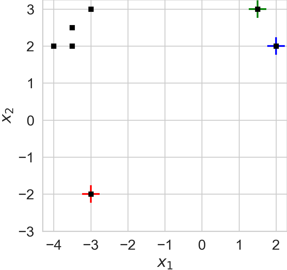
Plot of the N=7 toy data examples (squares) and K=3 initial cluster locations (crosses).
Problem 2a: Find the optimal one-hot assignment vectors \(r^1\) for all \(N=7\) examples, when given the initial cluster locations \(\mu^0\). This corresponds to executing step 1 of K-means algorithm. You should also report the value of the cost function \(J(x, r^1, \mu^0)\).
Problem 2b: Find the optimal cluster locations \(\mu^1\) for all \(K=3\) clusters, using the optimal assignments \(r^1\) you found in 2a. This corresponds to executing step 2 of K-means algorithm. You should also report the value of the cost function \(J(x, r^1, \mu^1)\).
Problem 2c: Find the optimal one-hot assignment vectors \(r^2\) for all \(N=7\) examples, using the cluster locations \(\mu^1\) from 2b. You should also report the value of the cost function \(J(x, r^2, \mu^1)\).
Problem 2d: Find the optimal cluster locations \(\mu^2\) for all \(K=3\) clusters, using the optimal assignments \(r^2\) you found in 2c. You should also report the value of the cost function \(J(x, r^2, \mu^2)\).
Problem 2e: What interesting phenomenon do you see happening in this example regarding cluster 2? What could you do about cluster 2's location from 2d to better fulfill the goals of K-means (find K clusters that reduce cost the most)?
Problem 3: Relationship between GMM and K-means
Bishop's PRML textbook Sec. 9.3.2 describes a technical argument for how a GMM can be related to the K-means algorithm. In this problem, we'll try to make this argument concrete for the same toy dataset as in Problem 2.
To begin, given any GMM parameters, we can use Bishop PRML Eq. 9.23 to compute the posterior probability of assigning each example \(x_n\) to cluster \(k\) via the formula:
Now, imagine a GMM with the following concrete parameters:
- mixture weights \(\pi_{1:K}\) set to the uniform distribution over \(K=3\) clusters
- locations \(\mu_{1:K}\) set to the initial locations \(\mu^0\) in Problem 3 above
- covariances \(\Sigma_{1:K}\) set to \(\epsilon I_D\) for all clusters, for some \(\epsilon > 0\)
Problem 3a: Show (with math) that using the parameter settings defined above, the general formula for \(\gamma_{nk}\) will simplify to the following (inspired by PRML Eq. 9.42):
Problem 3b: Compute the value of \(\gamma\) for all \(N=7\) examples when \(\epsilon = 1.0\)
Problem 3c: Compute the value of \(\gamma\) for all \(N=7\) examples when \(\epsilon = 0.1\)
Problem 3d: What will happen to the value of \(\gamma\) as \(\epsilon \rightarrow 0\)? How is this related to the K-means results from Problem 2?
Problem 4: Jensen's Inequality and KL Divergence
Skim Bishop PRML's Sec. 1.6 ("Information Theory"), which introduces several key concepts, including:
- Entropy
- Jensen's inequality
- KL divergence
Specifically, consider the negative logarithm function: \(f(a) = - \log a\), for inputs \(a > 0\). Recall that \(f(a)\) is a convex function, because its second derivative is always positive:
Now, assume the following quantities are known:
- Candidate input vector \(\mathbf{a} = [a_1, \ldots a_K]\), where each entry can be any positive value: \(a_k > 0\).
- Probability vector \(\mathbf{r} = [r_1, \ldots r_K]\), which are \(K\) non-negative values that sum to one: \(\mathbf{r} \in \Delta^K\).
Then, we have the following lower bound using Jensen's inequality (see PRML textbook Eq. 1.115), when specialized to the negative log (which only takes positive inputs):
We can visualize this bound in the following figure, using two selected points \(a_1 = 0.1\) and \(a_2 = 7.2\).
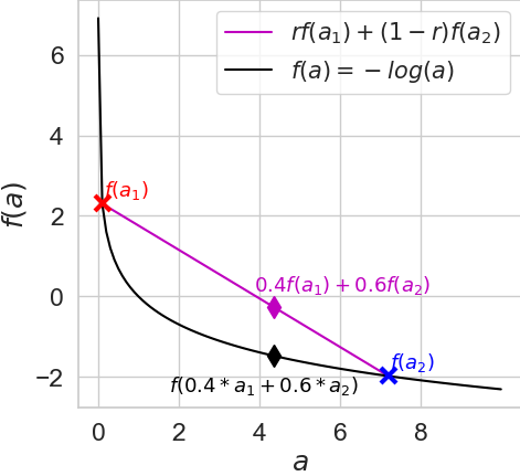
Plot of our convex function of interest ("f", black) and its *linear interpolation* (magenta) between outputs that correspond to two inputs "a1" and "a2". Clearly, function f is a *lower bound* of its interpolation (magenta)
Problem 4a: Using Jensen's inequality defined above, argue that if we consider any two Categorical distributions \(q(z)\) and \(p(z)\) that assign positive probabilities over the same sample space, then their KL divergence is non-negative. That is:
where we define random variable \(z\) as a one-hot indicator vector of size \(K\), and define distributions \(q\) and \(p\) in terms of all positive probability vector parameters \(\mathbf{r} \in \Delta^K_+\) and \(\mathbf{\pi} \in \Delta^K_+\). Here \(\Delta_+^{K}\) denotes the set of \(K\)-length vectors whose sum is one and whose entries are all strictly positive.
where the vector \(e_k\) denotes the one-hot vector of size \(K\) where entry \(k\) is non-zero.
Note: it is possible to prove the KL is non-negative even when some entries in \(r\) or \(\pi\) are exactly zero, but this requires taking some limits rather carefully, and we want you to avoid that burdensome detail. Thus, here we consider \(r\) and \(\pi\) as having all positive entries.